QGIS algorithm for natural shadow modelling.
Introduction
Modelling natural illumination is quite difficult in software for digital cartography. Yes, we do have hillshading algorithms, but despite the name they do not produce true shade. Hillshade routines colour the terrain according to exposition towards the sun (white for directly exposed and black for unexposed areas), but they do not model the light path. There are no shadows in hillshades. As a result, a canyon floor will be rendered the same way as a wide valley, which impedes the perception of depth. Hillshades often have a feeling of “elephant skin”, as if the Earth surface were wrinkled by long term cosmetic abuse.
Simple hillshade vs natural shadows: slide to compare
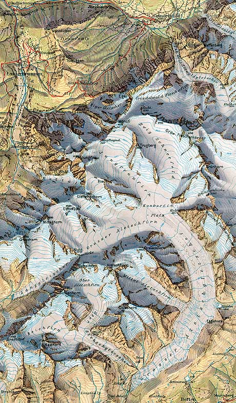
Compare these two images: shadows are not just nice, they enable better understanding of the terrain. Today, cartographers typically turn to 3D software, such as Blender, to obtain the effect of natural lighting (see for example scottreinhardmaps.com). Historically the effect was achieved by hand (figure below).

Jungfrau range (European Alps) by E. Imhof (see on reliefshading.com.
But, why should we drop all benefits of georeferenced environment and revert to software which can’t handle geographical data? It is not that difficult to simulate natural light, provided that we do not expect the same level of quality as in dedicated 3D doftware.
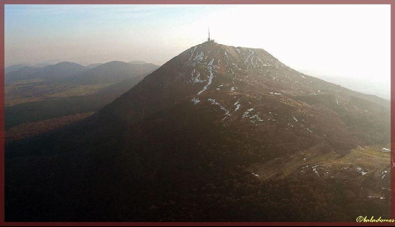
I have developed a short algorithm to simulate incident light over digital terrain models, namely the shadows it should produce. Rather than simple yes/no format, shadows are represented as depth values. In natural environment, there is a considerable difference between two metres deep shadow, as behind a small mound and hundreds of metres deep shadow, behind a cliff. Taking care of such nuances can help as to get closer to the refined effect of handmade hillshades.

Deep shadow below Puy de Dôme, France (© baladomes.com).
Algorithm
For those interested in the code behind my solution, these are the two crucial lines:
import numpy
shadows = elevations - numpy.maximum.accumulate( elevations )
The accumulate function takes care that values in the (numpy) array which stores the elevation model would only increase, from the beginning of the array to the end. Imagine walking over a mountain, along a path which is constantly winding upwards and downwards. If you would like to move only upwards, you would need to fill all valleys with soil or water. The accumulate function does just that, it simulates a cascading terrain profile where we can travel either upwards or over a flat terrain. Filled portions of the terrain become shadows if you imagine the sun shining into a flank of a mountain. Shadow depth is calculated by subtracting the cascading model from the actual terrain height.
from math import tan, radians
tilt_factor = tan(radians(sun_angle)) * pixel_size
tilt_matrix = tilt_factor * (indices_x + indices_y)
To simulate the vertical angle from which the sun is shining over the terrain, we rather tilt the entire elevation model. That is, we construct a sloping surface and the drape the terrain over it. Indices in the line above can be understood as distance values where the size of pixel is one. They increase from the corner (or the border) closest to the sun position. Note that we decompose distances on x axis and on y axis components: let’s pretend these are vector components (see the previous post on vectors and hillshades).
The rest of the algorithm is rotating the elevation model in different directions to simulate the entire 360 degree orbit. I’ve also included a smoothing function as the raw result tends to be very pixelated. The function is adapted from the Topographic position index algorithm.
You can see the algo in GitHub repository: QGIS-raster-sahding.
Using the algorithm and styling the output
The shading algorithm is used as a Processing script for QGIS 3 and is installed as usual (figure below). It will appear under Scripts » Raster terrain analysis » Natural shading in the Processing toolbox.

The input for the algorithm is a digital elevation model and the output is a “shadow map”. The result will be smoothed by default (otherwise there is a nasty pixelisation effect). Other parameters should be self-explanatory (sun direction and vertical angle).
The most important issue is limited handling of large datasets, because of numpy raster processing library, which is limited by the available live computer memory. Large rasters, if opened, will saturate live memory (raster size at which this effect may be noticed depends on your machine…).
The output will provide information on the depth below the closest sun ray for each pixel in a raster DEM. These values can be used to produce gradients of shadow tones, as opposed to uniformly dark surfaces. The best effect is made, as for usual hillshade models, when superimposing several layers in transparency mode.
Natural shadows work best where hillshades tend to produce the “elephant skin” effect; my first example is errored and gullied relief in Istria, Croatia. Here, I’m using an elevation model styled with hypsometric colours, overlaid with a hillshade model and a shadow model.
Rugged relief of Istria, Croatia and Slovenia
See how shadows introduce a feeling of depth? Now, simple black/grey shadows would be problematic as they could easily occlude detail in valleys. Or, if too transparent, they would just add some mist, without introducing much perceptual improvement. The algorithm for natural shadow modelling, however, provides information on shadow depth, which enables to fine tune the effect. Shallow shadows should be less strong, as we can suppose a stronger impact of light dispersal in such areas. Here, I’ve set different intensities of grey and different levels of opacity for five classes between zero and minus 400 metres. Typically you would also need to completely eliminate shadows less than 2 or 3 metres in depth (opacity = 0%), as they tend to encroach ridgelines and hilltops.
Shadow intensities are controlled by both colour and transparency for each depth class.
One last example, Požega valley in Croatian part of Pannonia:
Conclusion
The algorithm for natural shadow modelling gives nice results, but beware that it’s still in the “proof of concept” stage. There are several technical problems to be tackled in the future (such as handling large rasters). Please feel free to report any problems/inconsistencies that may arise.
Download
The script can be downloaded directly or from GitHub repository. Problems and issues can be signalled in the same repository.
Update, January 2020: the algorithm is now available as native QGIS plugin.
Happy mapping!