Hillshade modelling is a standard form of terrain representation in cartography. The idea is to simulate lighting of a terrain from a certain direction (or multiple directions). The method is well known and constantly improved in GIS – as means of cartographic representation. It seems, indeed, difficult to imagine spatial analysis on shadows.
However, hillshading is much used for analysis of Lidar data, usually when these are represented as gridded elevation model. The concern is not to render the model lifelike and aesthetically pleasing; on the contrary, images produced can be quite bizarre as they are tweaked to yield maximum contrast. Shadows are used for detection of topographic features. This brings a new issue : is there a (relatively) optimal way of shadowing the terrain, or are we to juggle with multiple hillshades, made form multiple directions?
Theoretically, such a model should exist for simple objects such as terrain features – no holes, no overhangs etc. Two lights from different directions (but not opposite to each other) should be enough to produce shadows on any topographical feature. But, combining these two (or more) hillshade models is not that obvious.
The problem of directedness
See what’s happening when two simple features are illuminated from north-east and north-west directions. The vertical feature (yes, these are wine corks) has its shadow shifted from one side to the other, but shadow of the horizontal feature will remain on the same side. Different alignments respond differently…
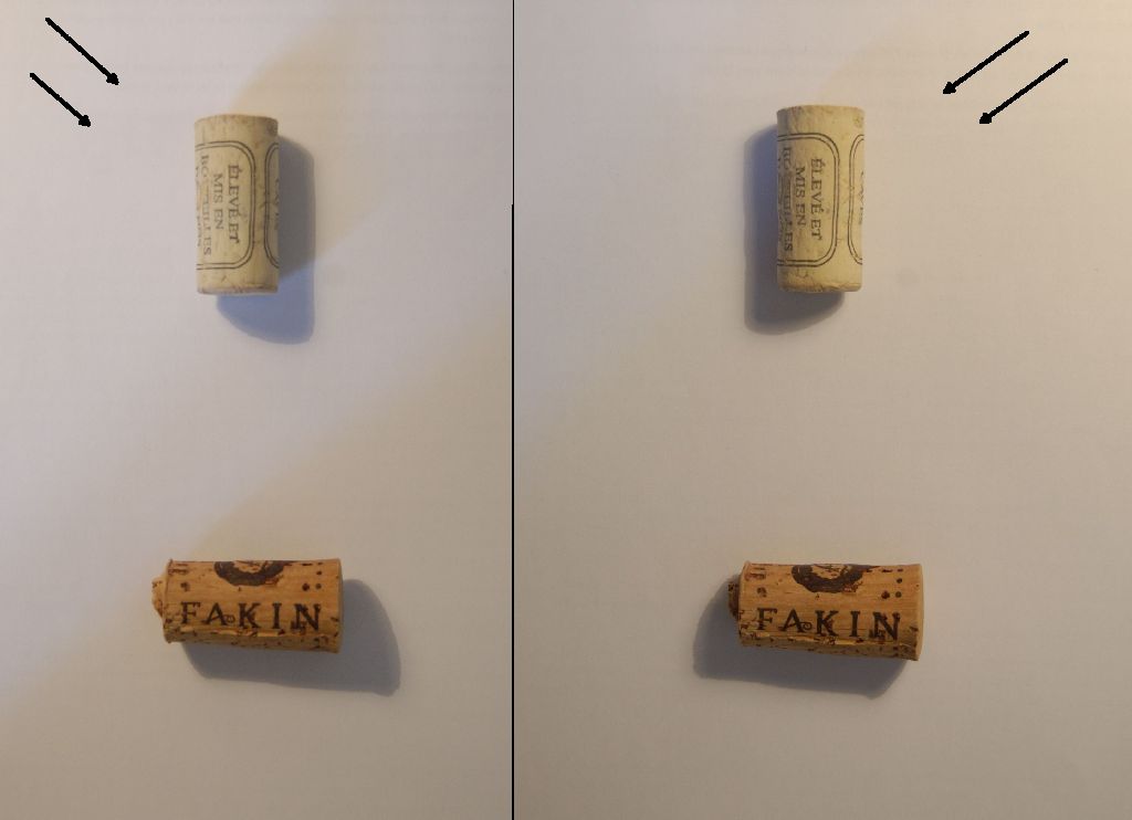
Vertical features will be better rendered if we calculate difference between the two models. What is a shadow in one model will become an illuminated patch in another one. But that approach will remove the impact of horizontal features. Their shadows remain on the same side: difference between two shadows is zero. In that case, addition of values will work much better.
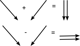
What this implies is that the sum of two hillshades (NW and NE) will effectively change the direction of light, as if it were on north. Subtracting them will have the effect of changing the light direction to either east or west. Hillshades can, then, be regarded as vectors, namely the X and Y component of usual two dimensional vectors. Therefore, all possible light directions can be calculated from two perpendicular hillshade models, given a constant light height. (We should add a third one to model all possible directions in a 3D sphere.)
Better hillshades?
Several conclusions can be made:
- Two perpendicular hillshades are all we need to model any hillshade direction for a given (i.e. constant) light altitude.
- Vector algebra can be used to combine hillshades and to extrapolate more complex indices.
- Multi-directional hillshade cannot be represented through a single variable, such as the grayscale. Combining two vectors will simply result in a new vector, as if we changed the light angle.
Therefore, bi-directional hillshade has to be represented through two independent variables. Hopefully we can see in colour, so this can be achieved by varying two colour scales … but that’s easier said than done. It takes a lot of messing around to achieve a readable result, an in particular the one that is more useful than a single grayscale image.
Footpaths can be a good case to test hillshading techniques. Their topographic trace can be very discrete, especially for those that are out of use and overgrown with vegetation (which typically interest archaeologists). Such paths can be traces of ancient pastoral movement or even abandoned roadways. The dataset used here is covering the western slope of Puy de Dôme above Clermont-Ferrand (France) which most likely bears traces of historical herding movement. Lidar data is offered free of charge for public use by CRAIG Auvergne.
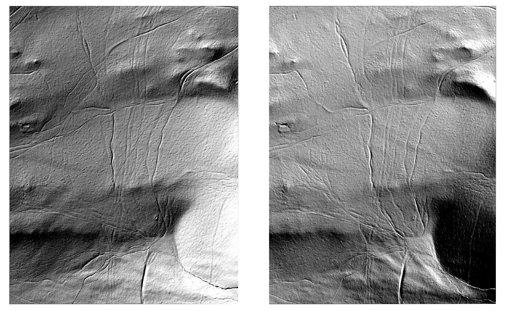
Meadow paths on Puy de Dôme, DEM of 50 cm resolution (© CRAIG Auvergne). Hillshades are modelled from north-western and north-eastern directions.
Two models with NW and NE direction are quite good, but still tend to accentuate different alignments. I’ve tried to overlay the two models, where the upper one (NE direction) is semi-transparent and coloured orange-brown to blue. The middle part of the coloured range is completely transparent. (The idea is that the warm colour lean to south and cold colour to north.)
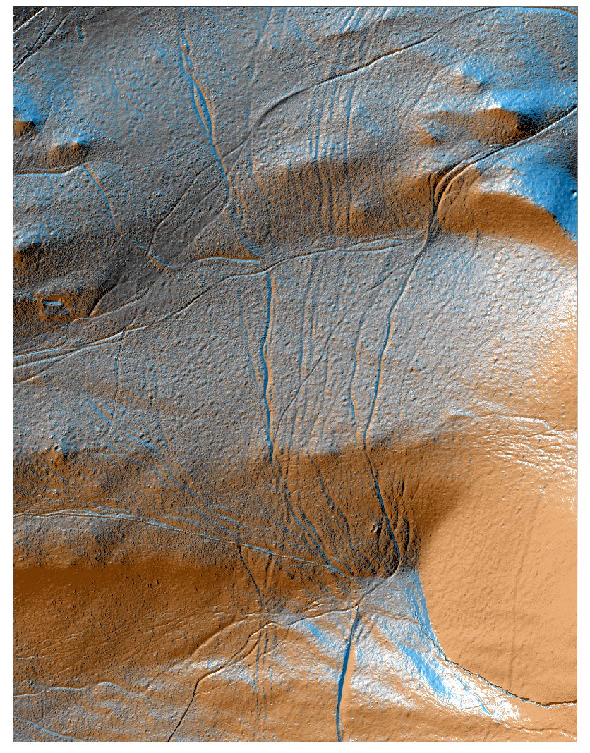
The result is not ideal, but it’s promising. Ideally, bi-directional hillshade should be combined in a colour image. But, combining colours is fussy… this is the result of a simple stack of our two hillshades:
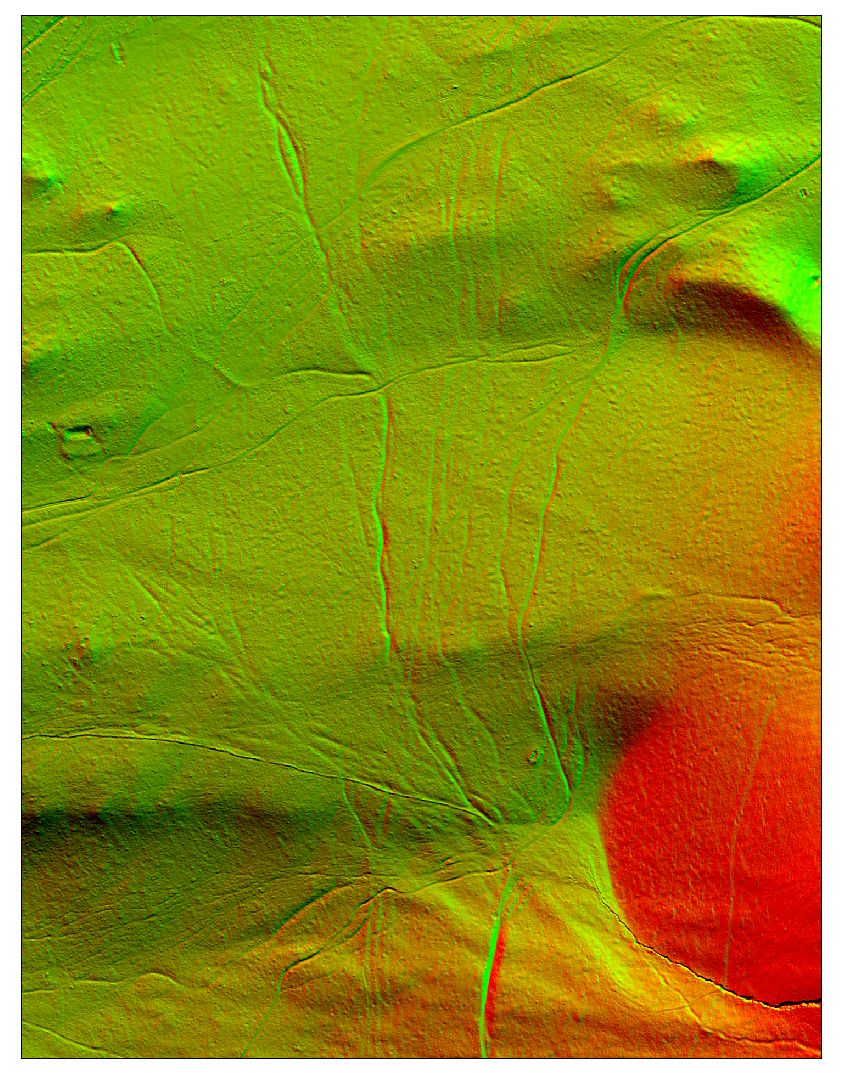
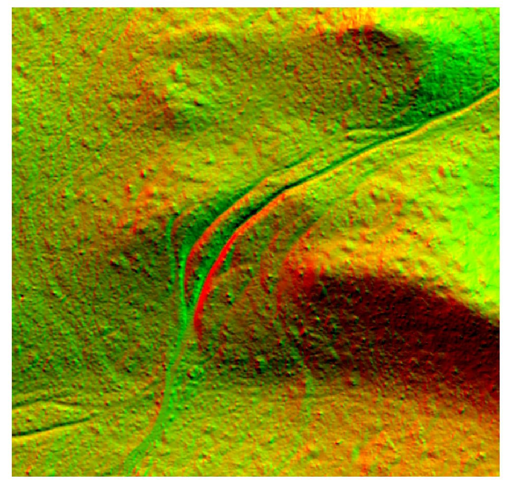
One hillshade is in the red band and the other is in the green band (blue band is empty). We should invert/stretch/edit band values to get a more pleasing colour combination… However, this procedure is effectively adding up colour values (red + green), which means that we will get the effect of vector operations. Take a look at the path below: the red colour is more intense on the western exposition than north-western, as we would expect from a hillshade calculated from that direction. Values now stretch east to west (red to green) and north to south (white to black) due to vectorised operations (!) So fussy…
I hope these ramblings would be of some use for those trying to understand hillshade models,
Happy mapping!