Starting with 0.9.2 version, QGIS Terrain shading plugin is equipped with the exquisit terrain shading algorithm, devised for terrain cartography by Leland Brown (refs. below). The algorithm can be described as a scaleless sharpening filter which permits to visualise height differences within a region without producing a flattened impression (the problem of the majority of other existing solutions). This magic is made possible by Fourier transform, a complex mathematical procedure which decomposes a series of values into repetitive, cyclical frequencies. This procedure is used for wave form analysis, for istance to extract and enhance specific frequencies from a music recording. Given the undulating, repetitive character of natural terrains, why not giving it a chance for natural terrains?
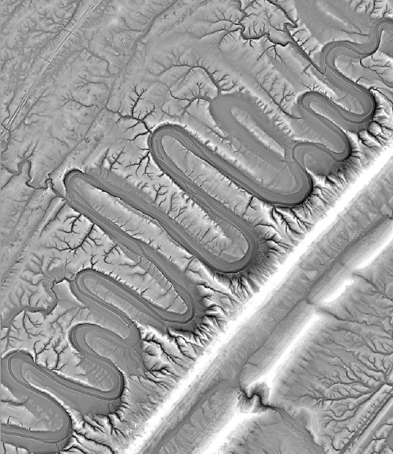
Massanutten Mountain, Virginia, USA (data from shadedrelief.com)
In theory, this can be used to extract landforms of specific sizes and to eliminate noise in the dataset. Banded, repetitive noise patterns that arise with radar or lidar datasets are an ideal candidate. That being said, texture shading does not rely on the extraction of frequencies, which would be highly complex. Its main goal is to profit from the scale-free character of the Fourier transform – which takes into the account the entire DEM, at once – to alleviate the well-known problem of common GIS filtering techniques. The vast majority of these is based on a moving window which jumps from cell to cell and takes into the account only their immediate neighbourhood.
The calculus in the frequency domain is beyond my math level; suffice to say that certain classic image filters can be reconstructed in the frequency domain and calculated far more efficiently than through standard window-based filters. One of those is Laplacian or sharpening filter:
H(u,v) = −(u² + v²)
where (u,v) are frequency vales for a cell (x,y) in a given raster. Note that (u,v) are a combination of all frequencies at such (x,y) point, which is why they need to be calculated for the entire width (u) and height (v). If we tweak this a bit such that
H(u,v) = −(u² + v² ) ^ alpha
and with alpha < 1, we end up with a strange function that gives us a half-filtered dataset, i.e. an elevation model that combines the original height relationships and some sharpening. Which is cool, as you can see below.
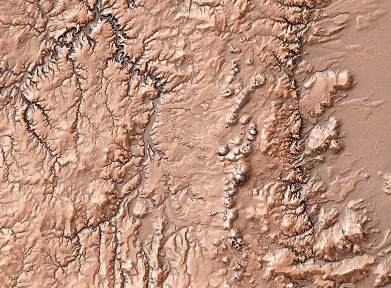
Volcano range of the Auvergne region, France (hillshade + texture shading + ambient occlusion; data by craig.fr)
What exactly does texture shading produce? While obtained figures reflect height relationships, they do not relate to a specific real-world phenomenon, such as actual height diffrences. Note that the visual effect of texture shading can be simulated by combining a large number of TPI models with increasing neighbourhood radius (Terrain Position Index). Therefore, texture shading can be considered as a sort of scalefree TPI.
As a final note, the argorithmic solution of the QGIS texture shading module is in many ways less sophisticated than the original formula. For instance, my solution does not handle well raster borders, and the math is significantly simplified. But it fits into some 30 lines of code, which is so cool for maintenance. The images are nevertheless stunning!
Resources
Leland Brown 2014. Texture Shading: A New Technique for Depicting Terrain Relief, www.mountaincartography.org
www.textureshading.com by Leland Brown
Terrain Texture Shader by Tom Patterson