Welcome visibility index algorithm, a.k.a. total viewshed, now available in QGIS Visibility analysis plugin. This metric informs us on the size of the visual field for any location across a given terrain, normally each pixel in a gridded digital elevation model (DEM). At first, visibility index resembles other terrain indices such as topographic position, terrain roughness, etc. However, the visual structure of the landscape is essentially a question of human (or animal) perception and has to be evaluated within a specific cognitive/perceptual framework. Rather than as a terrain quality, I like to think of visibility index as a model of visible scene quality.
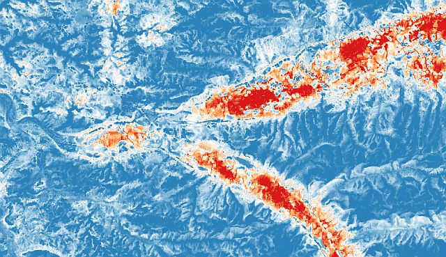
Visibility index for two river valleys: note high exposure of valley bottoms.
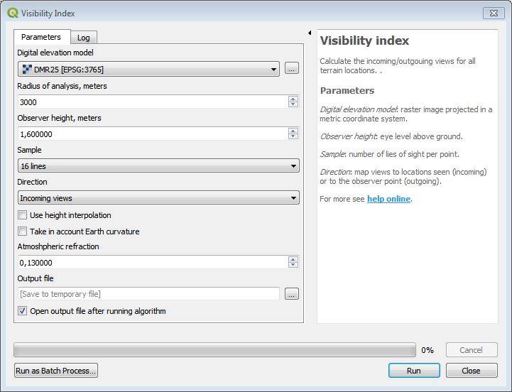
Visibility index is calculated as the ratio of positive visual connections: 1.0 or 100% implies that a point can be seen from all of its neighbours. In fact, we have two options when mapping these positive views. The first one is to assign the value to seen locations, which can be termed as incoming views. This is equivalent to cumulative viewshed (see my previous post). The second option is to map positive views to observer locations, which will register the size of observed surface. These are, then, outgoing views. View direction parameter can therefore be used to distinguish between visual exposure of terrain features and the visual coverage from each terrain location.
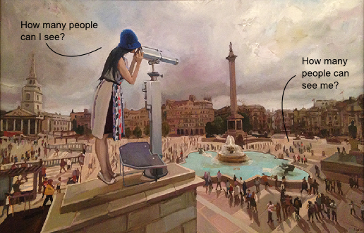
Visibility is not reciprocal: we can choose to model either the observer’s perspective, or the observed one’s perspective (painting by www.nadiatsakova.com).
The thing with visibility index is that it takes days and weeks of computing (see for instance Gillings 2015 who reports 300 hours of heavy calculation). Using standard GIS algorithms, you’re lucky if it takes only overnight! The reason is in the complexity of visibility calculations. Suppose that it takes 1 second to produce a single viewshed: for a 5 million pixel DEM (which is not large at all) this amounts to 1300 hours of computing.
These are serious algorithmic problems which are not easy to solve. I’ve coded a solution which a) eliminates calculation redundancy and b) takes the maximum advantage of spatial correlation of geographic data. It works as follows.
Untangling lines of sight for multiple viewshed calculation.
A typical viewshed is calculated by projecting lines of sight form an observer point in such a way as to touch all pixels within the specified radius. That procedure can be broken down in two operations: 1) line tracing and 2) pixel height evaluation. In case when observer points occupy the centre of individual pixels, the set of radiating lines can be (and should be) exactly the same for each point. If a certain line of sight starting in a pixel of row 10, column 12 is finishing in a pixel row 45, column 46, then for the observer on (20, 22) a corresponding line will finish in pixel (55, 56). We translate the coordinates by 10. Now, when all possible lines of sight describe same translations for all other pixels in a grid, we can apply each line of sight to all pixels simultaneously (rather than to repeat the procedure for each observer point). We’ve halved (at least) the calculation complexity.
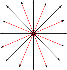
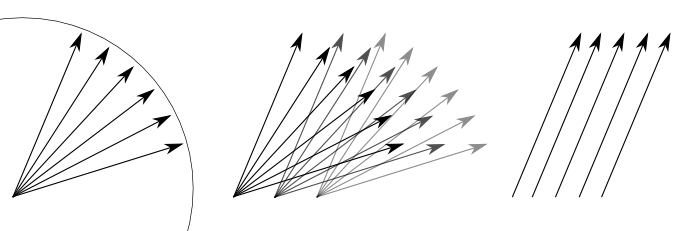
Sampling lines of sight: 16 lines.
The second optimisation relies on spatial correlation of typical DEM elements. Think of two adjacent pixels in a DEM: their values will most likely be very similar. Only in the case of standing architecture or very steep cliffs can we expect abrupt changes. Therefore, we can safely sample only a fraction of pixels and still obtain realistic visibility index. However, if these sampled pixels correspond to observer locations, we will be left with important discrepancies between pixels that have been analysed and those that were left out. This is especially problematic for ridgetop locations where sight direction and coverage vary significantly. A better approach is to sample lines of sight so that all pixels get equal coverage with, say, 8 lines of sight. Even such a low number obtains a surprisingly accurate result. As we raise the number of these lines, the outcome will slowly converge to a model produced with full range viewshed analysis. I’ve implemented 8 to 64 lines samples, to satisfy all levels of precision.
So, how long does it take? On my old and tired computer, with no CPU/GPU optimisation or whatever, it takes some 25 minutes for a 30 million pixel DEM (default parameters: 16 lines sample and 3 km radius). Not really a blink of an eye, but reasonable at least: these are viewsheds for 30 million observers!
The algorithm is based on Numpy library which can itself be optimised, but I havent’t yet ventured into these grounds: to be continued… Anyway, here it is, the first usable and reasonably efficient visibility index algorithm out there :).
Bibliography
M. Gillings 2015: Mapping invisibility: GIS approaches to the analysis of hiding and seclusion. Journal of Archaeological Science 62.
T.Brughmans, M. van Garderen, M.Gillings 2018: Introducing visual neighbourhood configurations for total viewsheds. Journal of Archaeological Science 96. open access.