Ambient occlusion is a concept developed in 3D modelling and visualisation which is used to evaluate the exposition to the ambient light of each model element. The idea is to simulate the diffuse, scattered light that bounces off various surfaces. Such light may not have an identifiable source, as for instance under overcast sky. Ambient occlusion models produce very realistic renderings which capture the dim light in tight spaces and corners (figure below).

Representing 3D volumes using ambient occlusion technique (pinterest.com).
Ambient occlusion is very promising for terrain visualisation, as well; a couple of scientific publications on the topic are listed below. The simplest and the most widely used approach assumes a homogenous distribution of light sources from all possible directions, as under a blanket of fog. In this case, the amount of the incident light is directly related to the portion of the visible radiant surface. This metric is called terrain openness and is expressed as the ratio of the sphere around each terrain point that is not occupied by the terrain itself. Note that we need to specify the radius of the sphere, and that the result will vary according to the reach of this radius. Sky-view factor is a variant of this method where we consider only the hemisphere above each point, hence the sky view. This approach has proven to provide a more intuitive output than openness, and is widely used.
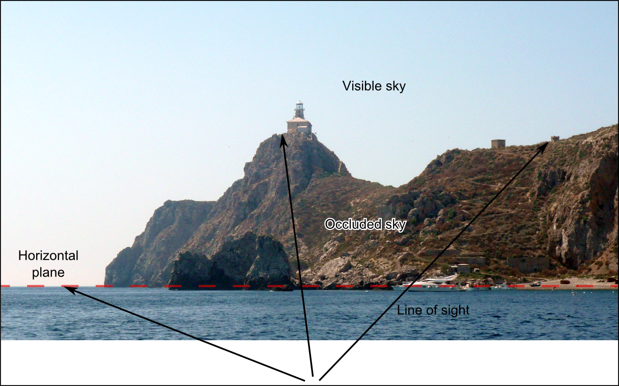
Real-life illustration of the sky-view principle (Palagruža island, Adriatic Sea, wikimedia.org).
In the image above, waterline approximates the horizontal plane for a sea level location (the photographer’s position). On the open sea, his/her sky view would be 100%, but here an island is blocking a small portion of the sky. The effect is inversely proportional to the distance from the island (the closer we get, the less light we receive). Terrain openness value, however, will never surpass 50% on the open sea, as only half of the surrounding sphere will remain unblocked. Openness values above 50% are nevertheless possible for ridgetop positions, such as the one occupied by the lighthouse in the figure above. Provided that we specify short sphere radius, say 100 meters, the light-blocking sea surface will appear significantly below the lighthouse.
Openness and sky-view factor are now available in the Terrain shading plugin for QGIS. As in other common approaches, these metrics are estimated with a sample of lines of sight, projected from each terrain element (a pixel in this case). As of writing, 8 lines are used. As a side-note, this plugin already features a shading algorithm inspired by the principle of ambient occlusion; the shadow depth method calculates the depth-dependant shadow translucency.
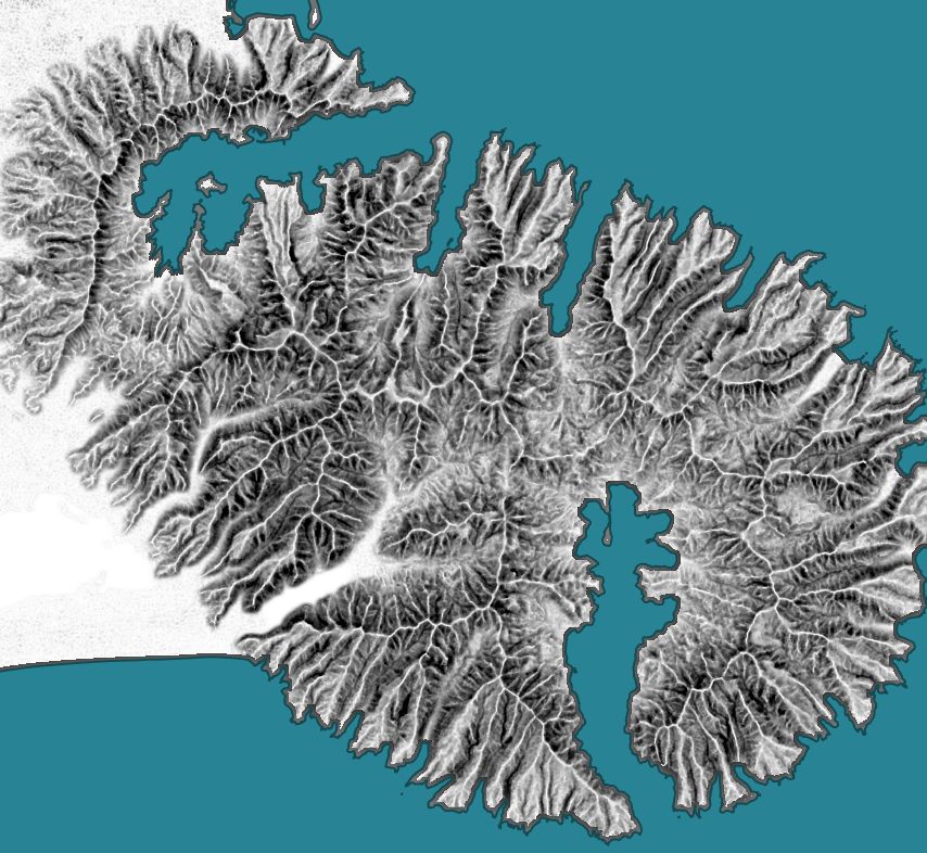
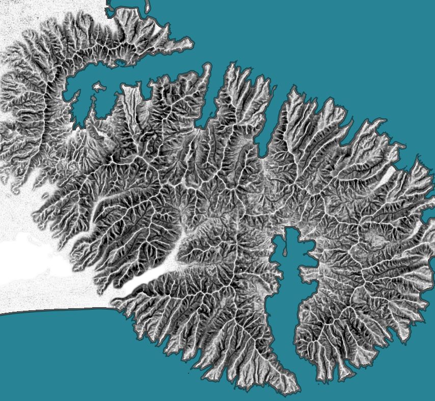
This simple sky-view factor shading of Banks peninsula (New Zealand) is ideally suited to represent the intricate ridge network which developed through erosion of the volcanic terrain. We can also add some shadow effect (using QGIS Terrain shading plugin) to enhance the impression of depth (even if the example below may be a bit exaggerated).
Refinement: calculations over an inverted DEM
If we observe carefully the images above, we may notice that the sky-view factor is more efficient for rendering ridgelines than valley bottoms and drainage channels. This is probably not a major issue, but let’s try to compensate for this effect.
In order to provide a better impression of valley bottoms, we need to invert the elevation model, as a glove, so that valleys become ridgelines and vice versa. That’s elementary, Sherlock would say, just multiply the elevation model by -1 (in QGIS raster calculator: my_dem * -1). We can now do all our analyses as usual.
Metrics obtained using this technique are called negative openness and, by analogy, negative sky-view factor. However, it’s just a hack which has no intuitive explanation, the result is not related to a real-world phenomenon.
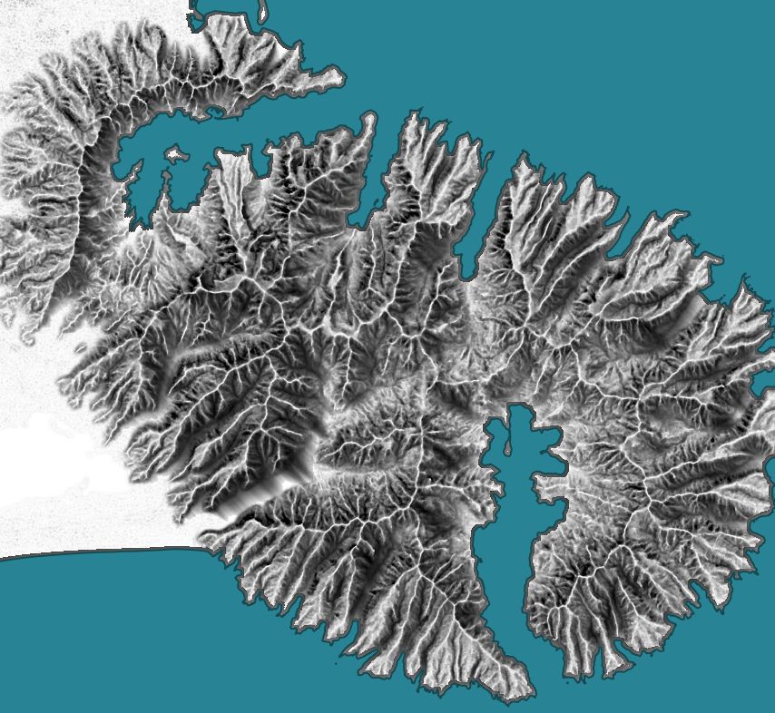
The above image shows the result of sky-view algorithm over an inverted DEM. Note the superior rendering of deep drainage channels, which now appear as fine black lines. The overall sharpness is also significantly improved. Unfortunately, the model doesn’t convey the feeling of depth, the terrain seems flattened and schematic.
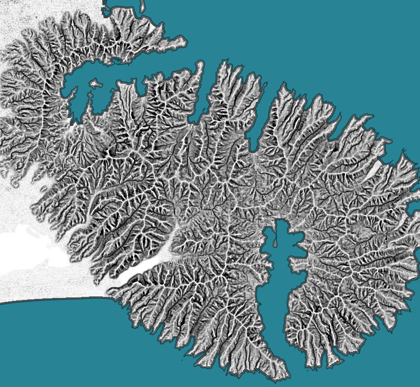
Combined positive and negative sky-view factor.
To obtain the best from both worlds, we can combine the usual sky-view factor with the negative one, as on the figure above. Here, the negative SVF is overlaid as semi-transparent layer using the “Overlay” blending mode (see screenshot below). Our SVF shading is now sharper and more detailed in low lying areas, while still preserving the ambient occlusion effect that produces the 3D feeling.
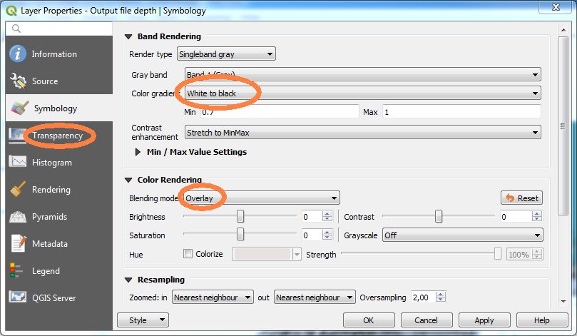
QGIS stlye used for the negative SVF overlay. Valleys are represented with an inverse scale (white to black) and superposed as a semi-transparent layer over the usual sky-view model.
Happy mapping!
Software
QGIS Terrain shading plugin, see at LandscapeArchaeology/qgis-terrain-shading/
Bibliography
K. Zakšek, K. Oštir and Ž. Kokalj 2011: Sky-View Factor as a Relief Visualization Technique. Remote Sensing 3(2), 398-415.Open access.
R. Yokoyama, M. Shlrasawa and R. Pik 2002: Visualizing Topography by Openness: A New Application of Image Processing to Digital Elevation Models. Photogrammetric Engineering & Remote Sensing 68(3), 257-265. Semantic scholar