Visibility analysis plugin for QGIS is prospering quite well. As of writing [2016], it counts some 20 000 downloads and a bunch of « votes », which means that at least several thousand people are using it. (Although, it does feel uncomfortable knowing that any potential error would risk a blame-storm ….)
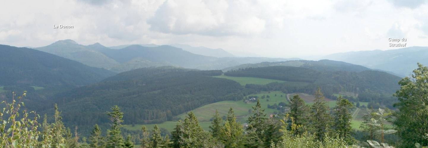
The new release brings a more polished algorithm and two options for horizon analysis. Horizon detection was, and still remains, rather problematic. On the conceptual level, the skyline has to be understood in terms of perception and not as a fixed terrain parameter. Consider the image below: there are many skylines in the mountainous landscape, progressively dissolving into the atmosphere. The most distant skyline might not even be visible at all, even if it would be rendered as “true horizon” by GIS. Sometimes we may be able to see a chain of mountains at distances above 100 or 200 km, but such views demand exceptional weather conditions. A book was recently published by William Malm (2016) on that particular issue.

Fig 1. A scene from Vosges mountains, France (Wikimedia commons, author “lybil”)
I do not find the “true horizon” analysis completely satisfactory for modelling real-life situations, particularly in open landscapes where atmospheric conditions restrain long distance visibility. In order to account for all potential, intermediary horizons, the QGIS viewshed plugin features an additional option for rendering “full horizon” (if the term is correct), i.e. all breaks in visibility patches for a given observing location. The idea is to be able to analyse and to filter those intermediary breaks that may become skyline under such and such conditions. That is not a trivial problem at all, but let’s leave the joy for some other occasion…
On the technical side, calculating the apparent horizon over a pixel grid poses some minor problems. The approach implemented in ArcGis (ref. below) apparently uses a set of arbitrary lines of sight that radiate from observer point, which could be problematic in terms either of precision (small number of lines of sight) or speed (large number of lines of sight). Lake and Ortega (2013) used GRASS r.viewshed in combination with a custom script which also projects an arbitrary number of lines of sight over a viewshed map. This means that the same analysis is made twice (lines of sight are projected first to obtain the viewshed raster and then for the horizon analysis), which is costly in terms of calculation time.
The algorithm implemented in the QGIS viewshed plugin examines all the height values for each line of sight in a same manner as for viewshed modelling and then registers either all horizon breaks or only the furthest (true) horizon break for each line. However, this does not guarantee a total consistency with viewshed output. Pixels are small blocks and we have to choose between testing the visibility towards their centre (or as close to the centre as possible) and testing the line of sight as it passes between the blocks. A particular line of sight passing between two pixels may be blocked, even if these pixels be modelled as invisible. Such cases are relatively rare, but they do occur and there is always some minor discrepancy between the modelled viewshed and modelled horizon.
Finally, unlike ArcGIS skyline module, the implemented algorithm does not force horizon line over visible areas that are cut off by the radius of analysis or by the extent of the elevation model.

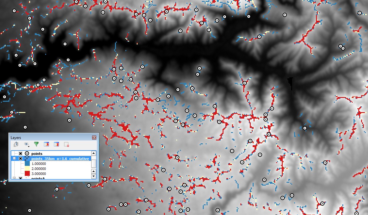
Figure 2. Cumulative horizon output
A new treat: cumulative horizon
Integrating horizon analysis into the core viewshed analysis enables an important speed gain. We are now able to do heavy calculation in a “reasonable” amount of time. I’m quite fond of cumulative horizon maps, i.e. the sum of all horizon models, similar to cumulative viewshed. It is usually higher ridges or other obstacles that tend to appear on the skyline from multiple locations in the landscape, which means that the analysis would reveal both, features that have a high overall visual impact and which at the same time tend to partition the space into distinct landscape zones (Fig. 2).
NB. To cite the current version (0.5.x) of QGIS visibility analysis refer to: JOSS article
Bibliography
ArcGIS skyline (N.D.). How Skyline works, desktop.arcgis.com
Lake, M.W., Ortega, D.A. (2013). Compute-Intensive GIS Visibility Analysis of the Settings of Prehistoric Stone Circles. In Bevan, A., Lake, M. (Eds.), Computational Approaches to Archaeological Spaces. (pp. 213-242). Walnut Creek, California: Left Coast Press.
Malm, W. (2016). Visibility, The Seeing of Near and Distant Landscape Features. Elsevier.