Introduction
The method of landscape chambers is used to delimit visually coherent zones in the landscape — which is not a trivial problem. The following tutorial presentes a practical, step-by-step guide for the generation of a simple model. For a more general discussion please check my landscape chambers article.
The method is based on intervisibility networks, which in their turn are segmented into cohesive groups. The idea is that such groups of visually connected observers appear in specific, visually integrated areas. Most commonly, such areas can be found in lower basins and valleys, and tend to be separated by higher relief. Plateau edges can also act as visual barriers.
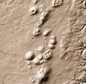
The example for the following tutorial comes from the volcanic range of Puys in France. Its topography is particularly interesting because volcanic cones represent rather weak visual barriers; we can indeed see and walk through the spaces between them. There are also several plateau edges to the east and west of the range. Delimiting visually coherent zones by hand would be a challenging and a highly subjective affair.
Tutorial
In order to follow this tutorial you will need QGIS software and Visibility Analysis plugin (which is installed as other standard QGIS plugins). The network analysis will be made with a dedicated script, called “Networks NX” and downloadable from https://github.com/zoran-cuckovic/QGIS-scripts. That page is also presenting steps for installing QGIS scripts. Note that the script is using Python’s Networkx library – if it is not available in your QGIS install, please follow the steps for installing Python libraries (where your library name is networkx). Now, let’s get our hands dirty!
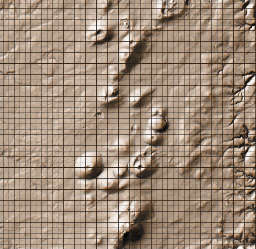
The first step is to produce a set of observer points. We can generate random points or a regular grid. I will rather start with a regular grid* of polygons, which will come as handy later on. Polygons, i.e. squares are 250 m large.
* The bold text can be typed in your Processing toolbox in order to find the corresponding tool.
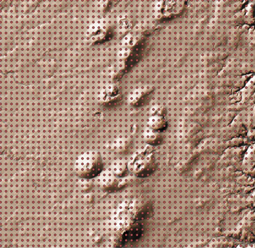
In order to obtain the required observer points, we will generate centroids for these polygons.
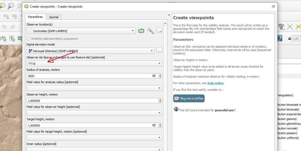
Next, we will use the Visibility Analysis routine called Create viewpoints in order to… do just that. Important : use the centroid ID number as your observer ID. Other parameters can be set according to your needs, but note that my observer and target size are the same. Otherwise, it would become messy (an observer who is looking from one height but is being seen at another height ?).
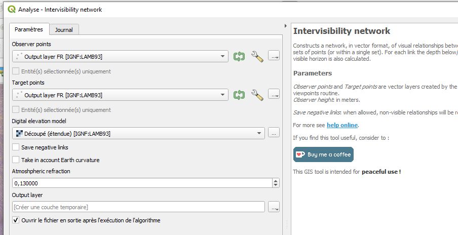
Crucial part, we will now calculate the intervisibility network. We are using the Intervisibility network module which is fed with a DEM and observer points. My DEM is of 25 m resolution, which is in most cases sufficient (for a landscape wide approach). Attention, the intervisibility network calculation is rather slow for massive data: anything above 10 000 points will put your patience to a serious test. (I have only 2 000 points for this tutorial).
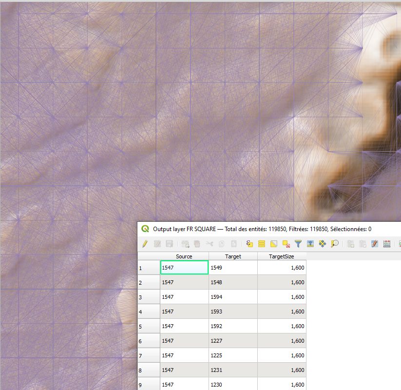
Let’s observe the result: a set of lines with IDs for observers and their view targets, as well as the info on target size. If a target is only partially seen (less than its full size), it can be filtered out, depending on your criteria for view quality.
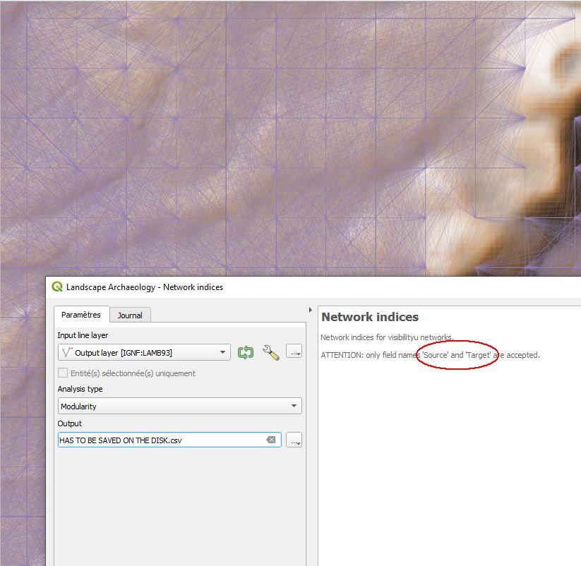
At this point we need to perform a network segmentation routine using the Network indices script.* Choose the “Modularity” option and save the result to the disk (temporary files do not work…). Note that the script is assuming that your vector layer contains columns named “Source” and “Target”; it will not work with other configurations.
* If the script bugs, see the first part of tutorial on installing the Networkx library in Python.
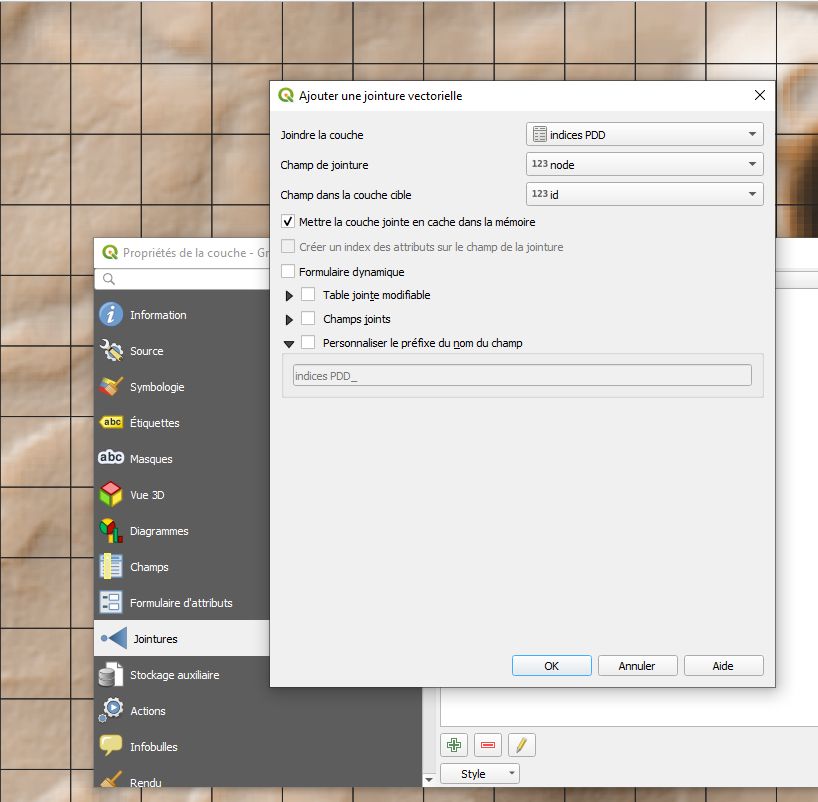
All that remains now is to link the produced data using table joins that we all love so much. Load the .csv file with the modularity values, and link it with the polygon grid that we produced at the very beginning. If you followed closely this tutorial, polygon IDs correspond to node IDs in the .csv table.
To finish, we will colour the polygon layer on the basis of assigned groups. QGIS has a very handy function for fusing together polygons with the same value, which produces the result below (cartography has to be left for another tutorial…).
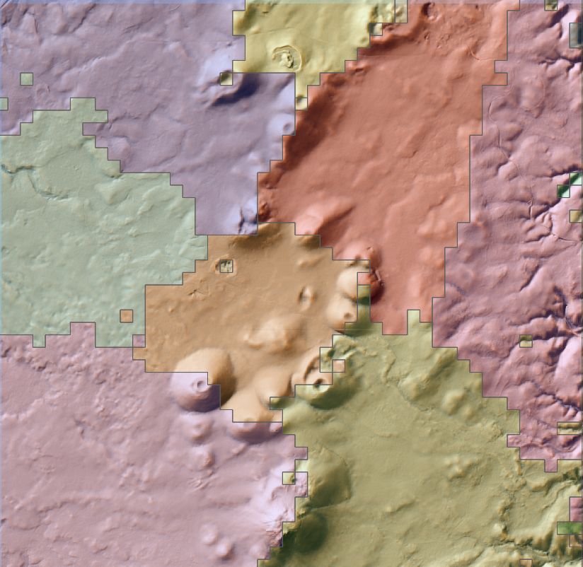
… and with borders only:
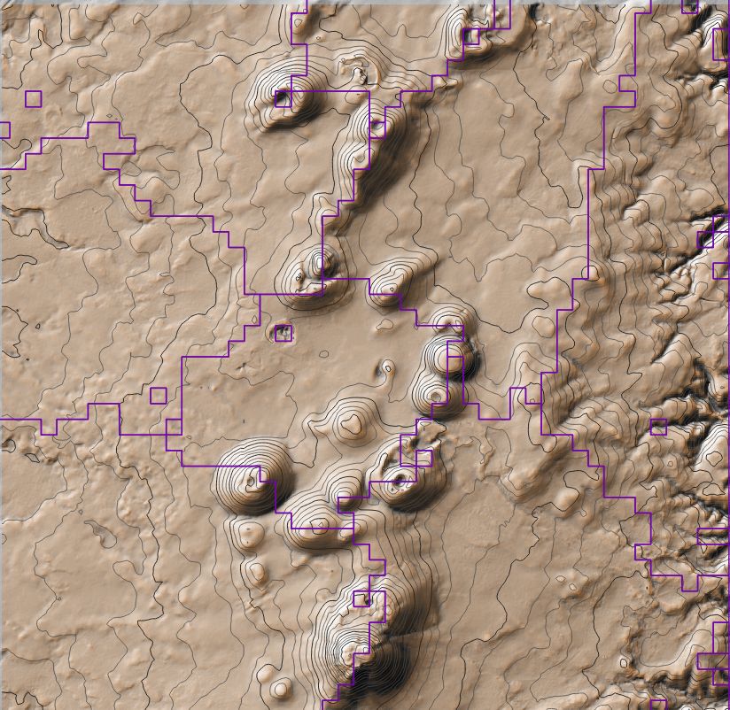
Note how the routine picked the small, circular space surrounded by volcanoes to the east and a plateau edge to the west. Plateau edges are separating chambers to the east and to the west, but only when their slopes are sufficiently pronounced; gentle slopes do not have this effect in the north-west and south-west.
There are many points that are worth discussing, such as observer density, view distance, the algorithm for graph segmentation…, but let’s keep this tutorial simple and practical. Do check the original article or drop me a word through the about page.
Happy mapping !