Topographic position index (TPI) is a method of terrain classification where the altitude of each data point is evaluated against its neighbourhood. In a nutshell, for each data point, i.e. a pixel in raster DEM, we calculate its height difference from the immediate neighbourhood. A detailed explanation can be found in the post on the TPI method. Here, I present a Python implementation of the TPI, for all those who wish to venture into custom filter programming.

Terrain position index (concavities are in blue and convexities in red). These are animal tracks and some human paths on a Lidar derived DEM.
The TPI method can easily be customised and experimented with in order to obtain that original result which will distinguish your work form other push-button solutions. We can play with window size or specific weight factors, for instance when window periphery should count less than the window centre. Such freedom can be very useful when fine tuning Lidar visualisations, for example.
In what follows, I will only provide the basic architecture for a TPI filter, based on the sliding window routine developed for numpy. In essence, TPI is just a kernel routine, which gathers information around each data point. At the same time it applies a weight factor, for instance to correct for the distance difference between diagonal pixels (touching by a corner) and orthogonal ones (touching by a side; below).
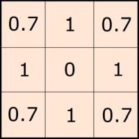
Standard TPI kernel (moving window) with distance correction
Below is a script that can be used in QGIS (open the Python console and just copy-paste the code) or run in pure Python.

Running the script in QGIS Python console
"""
Topographic position index for elevation models,
a mock script to be tuned according to you needs.

All comments are welcome at landscapearchaeology.org/2019/tpi
by Zoran Čučković
"""

import gdal
import numpy as np

# -------------- INPUT -----------------
elevation_model ="__path__to__my__dem__"
output_model = "__path__to__my__output__file__"


# ----------  create the moving window  ------------
r= 5 #radius in pixels
win = np.ones((2* r +1, 2* r +1))
# ----------   or, copy paste your window matrix -------------
# win = np.array( [    [0, 1, 1, 1, 0]
#                      [1, 1, 1, 1, 1],
#                      [1, 1, 0, 1, 1],
#                      [1, 1, 1, 1, 1],
#                      [0, 1, 1, 1, 0]  ])

# window radius is needed for the function,
# deduce from window size (can be different for height and width…)
r_y, r_x  = win.shape[0]//2, win.shape[1]//2
win[r_y, r_x  ]=0  # let's remove the central cell

def view (offset_y, offset_x, shape, step=1):
    """
    Function returning two matching numpy views for moving window routines.
    - 'offset_y' and 'offset_x' refer to the shift in relation to the analysed (central) cell
    - 'shape' are 2 dimensions of the data matrix (not of the window!)
    - 'view_in' is the shifted view and 'view_out' is the position of central cells
    (see on landscapearchaeology.org/2018/numpy-loops/)
    """
    size_y, size_x = shape
    x, y = abs(offset_x), abs(offset_y)

    x_in = slice(x , size_x, step)
    x_out = slice(0, size_x - x, step)

    y_in = slice(y, size_y, step)
    y_out = slice(0, size_y - y, step)

    # the swapping trick
    if offset_x < 0: x_in, x_out = x_out, x_in
    if offset_y < 0: y_in, y_out = y_out, y_in

    # return window view (in) and main view (out)
    return np.s_[y_in, x_in], np.s_[y_out, x_out]

# ----  main routine  -------

dem = gdal.Open(elevation_model)
mx_z = dem.ReadAsArray()

#matrices for temporary data
mx_temp = np.zeros(mx_z.shape)
mx_count = np.zeros(mx_z.shape)

# loop through window and accumulate values
for (y,x), weight in np.ndenumerate(win):

    if weight == 0 : continue  #skip zero values !
    # determine views to extract data
    view_in, view_out = view(y - r_y, x - r_x, mx_z.shape)
    # using window weights (eg. for a Gaussian function)
    mx_temp[view_out] += mx_z[view_in]  * weight

   # track the number of neighbours
   # (this is used for weighted mean : Σ weights*val / Σ weights)
    mx_count[view_out] += weight

# this is TPI (spot height – average neighbourhood height)
out = mx_z - mx_temp / mx_count

# writing output
driver = gdal.GetDriverByName('GTiff')
ds = driver.Create(output_model, mx_z.shape[1], mx_z.shape[0], 1, gdal.GDT_Float32)
ds.SetProjection(dem.GetProjection())
ds.SetGeoTransform(dem.GetGeoTransform())
ds.GetRasterBand(1).WriteArray(out)
ds = None
The script is using both, window geometry (square, circle etc.) and window weights which are applied to individual values. Geometry is modelled by setting unwanted window parts to zero, while weights should be non-zero values. Note that zero values are simply skipped as if non-existent, which will not happen with, say, weight = 0.00001.
It is not difficult to create a window on the fly:
r = 5 #radius in pixels
win = np.ones((2*r +1, 2*r +1)) #square window, all values are 1
win[r, r] = 0  #skipping the central cell
For Gaussian window weights: see numpy documentation.
However, I find more useful (and intuitive) to hard-code window definitions. This is very handy when comparing results on different datasets – there can be no error when the window is specified cell by cell. We can also keep a diary with window definitions that work best, like:
- Fine 5×5 filter :
0, 0, 0.5, 0, 0 0, 0.5, 1, 0.5, 0 0.5, 1, 0, 1, 0.5 0, 0.5, 1, 0.5, 0 0, 0, 0.5, 0, 0 - Aggressive 5×5 filter
0, 1, 1, 1, 0 1, 1, 1, 1, 1 1, 1, 0, 1, 1 1, 1, 1, 1, 1 0, 1, 1, 1, 0 - A totally skewed filter for detecting linear patterns:
              0, 0, 0, 0.5, 1
              0, 0, 0.5, 1, 0.5
              0, 0.5, 0, 0.5, 0
              0.5, 1, 0.5, 0, 0
              1, 0.5, 0, 0, 0
Danger in this approach lies in the assumption that the central data point is in the geometric centre of the kernel window. For this to be true, dimensions of the window should be in odd numbers. For instance, in 3×3 window, the central pixel is at (1,1) position. In a 4×4 window, the centre falls between cells, which doesn’t work! Therefore, be sure to count your pixels.
Larger windows may become unwildely; in that case you can always use the on-the-fly method, as above.