[This is the third post in my series on hillshades: previous ones were on the functionality of QGIS Terrain Shading module and some ramblings on the combination of multiple hillshades.]
In general, the use of hillshades in GIS is to make pretty visualisations, for mapping or for visual detection of terrain features, as for instance in archaeology or geomorphology. However, even if prettiness is the main criterion that we may care of, this doesn’t mean that we should skip the concepts that are involved. In fact, hillshades seem to be rather poorly understood, even in scientific literature. What is hillshade, in the first place?
Hillshade is not a model of what a terrain would look like when viewed from above: it’s a model of only one light component. Namely, hillshade represents the immediate light reflectance. Therefore, the result on its own gives an impression of wrinkled aluminium foil, the appearance of which is dominated by the immediate light reflectance alone.
Single hillshade
To get a more realistic terrain shading we need to a) combine the hillshade with other models and b) isolate hillshade components that we’re interested in. Here, we will combine hillshade with ambient occlusion, which models the diffuse light.
Ambient occlusion: the base layer. Massanutten Mountain, Virginia, USA (shadedrelief.com).
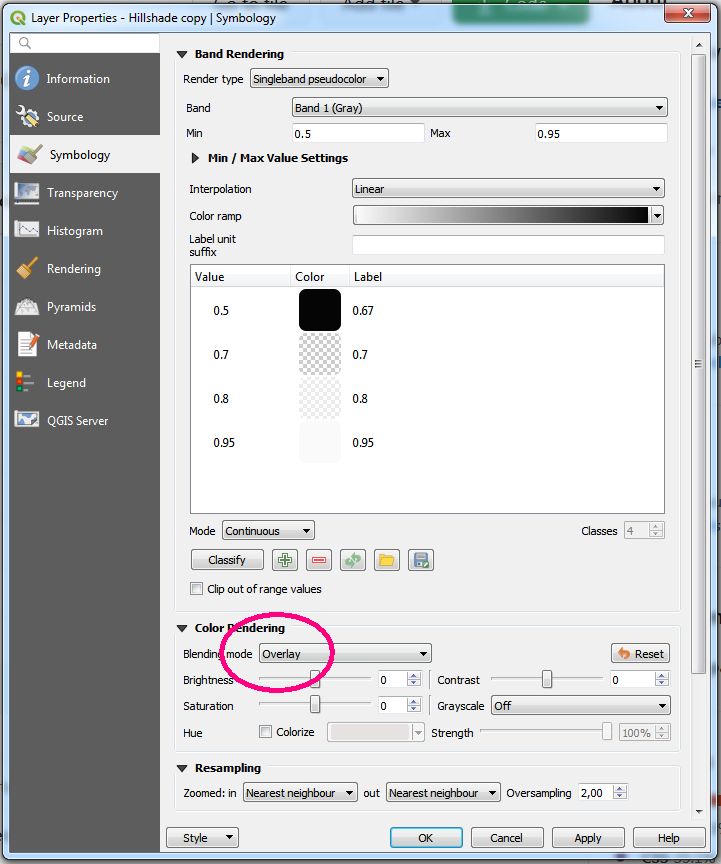
Light source for the ambient occlusion is undefined, the light comes from all directions of open sky (but always from above). We will now use hillshade to introduce the reflectance effect of direct sunlight (standard, NW sun direction is used). All grey areas that have average reflectance are removed: see the figure below.
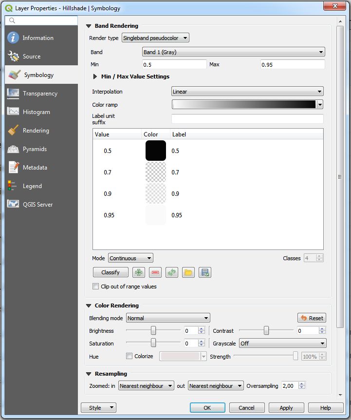
This colour ramp is removing the average reflectance component, i.e. the grey zone. Values between 0.7 and 0.9 are completely transparent.

Ambient occlusion model overlaid with a hillshade.
This filtered hillshade is then overlaid on ambient occlusion model (above). The diffuse light component is still dominant, but it’s certainly more readable once we’ve introduced the reflectance. The problem of this method is that it tends to produce dull grey patches on steep slopes. These areas have both, high reflectance and low diffuse light levels, i.e. they become uniformly white in the hillshade and uniformly black in the occlusion model, which doesn’t combine well. In order to counter this effect, I’ve used two levels of white, with varying transparency values (see the colour ramp above).
This is, then, the principle: isolating light components that interest us before delving deep into colour tweaking and such. (Which I’m not really good at …)
Multiple hillshades
Combining hillshades seems to be a major mystery. Indeed, two or more stacked hillshades would only produce another hillshade; because of some strange vector operations we can’t achieve any qualitative improvement. For the same reason, two hillshades with perpendicular light source suffice to model all possible light directions: anything more than that is simply redundant. (A third model may be introduced to handle the vertical position of the light source, but that’s rarely needed for relief mapping).
However, we can combine as many light components as we wish, provided that these do not interfere too much with each other. This can be done as above, by isolating specific reflectance values and masking others. That being said, the mathematical formula for hillshade normally takes into account the slope perpendicular to the light source, which means that the result is always somewhat influenced by the light component coming from the perpendicular direction (see my previous post). In QGIS Terrain Shading module, this perpendicular component can be removed, by setting the lateral exaggeration factor to zero.
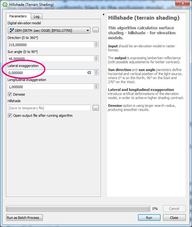
Removing the lateral component for a multiple hillshade model
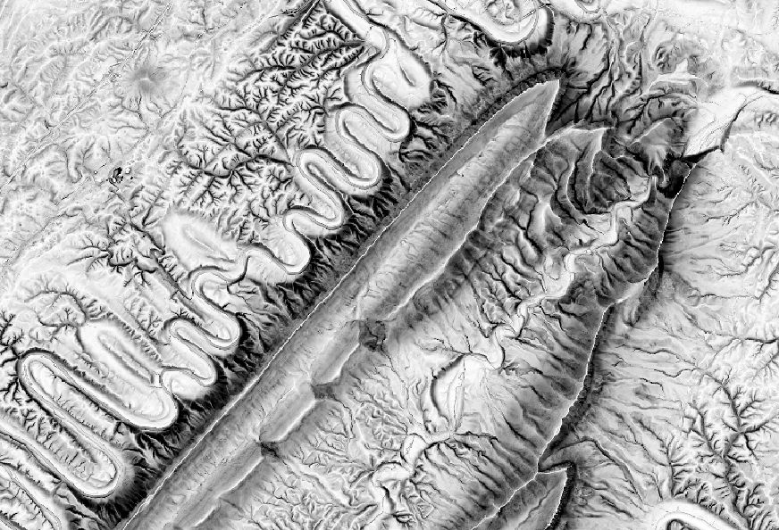
We will now follow the same principle as above, one hillshade is chosen as the base layer, here the one made from the NW direction, and the perpendicular hillshade, from the NE direction, will be the additional component. We need to remove all the grey areas and to conserve only the high and/or low reflectance values for the NE component: I’ve added two transparent stops to ensure complete transparency between 0.7 and 0.75. Note that the blending mode is set to overlay, this produces the best results.
Styling the second component for a bidirectional hillshade
The result is now much richer than a single hillshade, but it’s also more difficult to control. There is some interference, especially on high slopes. In any case, this is the theoretical maximum of information that we may get for a given height of the light source (here 45 degrees). We can still introduce models made for other directions, but with very restricted value ranges to highlight specific terrain exposures.
Bidirectional hillshade is, in theory, revealing the maximum information.
Wrap up
Hillshade is probably the most widely used method for terrain visualisation. Its result is rather intuitive, but its handling not so. In this post, I’ve discussed some principles which are not aesthetical, but rather conceptual. Hillshade is about modelling light, namely reflected light, which is only one component among several that are required to model a realistic scene. In order to do so, hillshade models should be broken down to different lighting components, which can be then be combined with other shading methods.