Contour lines have become a commonplace, unassuming companion of our cartographic outputs - GIS has made us forget their visual potential. Already in the 19th century cartographers experimented with shaded contours, but the technique has become known as the Tanaka method, after Japanese cartographer Kitiro Tanaka (Kennelly 2016, wiki.gis 2017). Even the cover page of Imhof’s seminal book sports a pile of shaded contours!

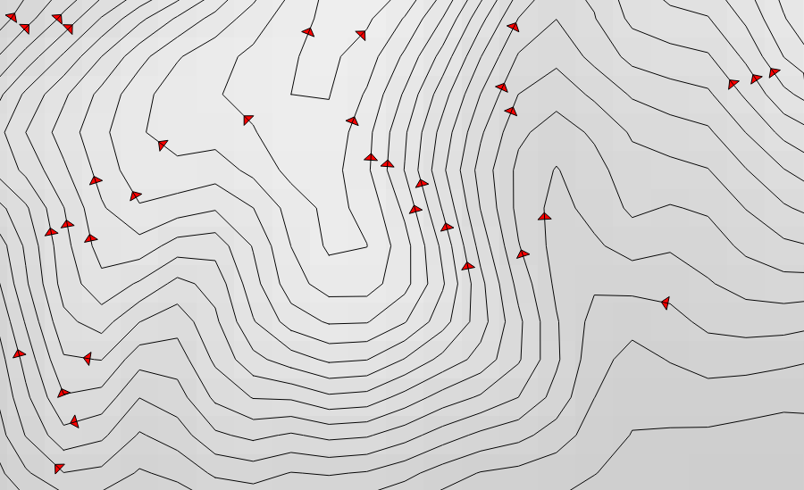
Shaded contour thickness and colour vary according to difference between the line direction and the light source direction. Lines perpendicular to the light are thicker than those parallel to it, while lines on “sunlit” slopes should be brighter than those on slopes under shadow. Such rendering adds the feel of the third dimension to the contoured map - without any actual 3D model.
A solution for achieving this effect has already been proposed by A. Graser a couple of years ago (link below). I’ve adapted the method for the newer versions of QGIS, and added a logic that permits to change light angle.
Contours
Contour shading requires consistent contour direction, that is, they should all be either clockwise or counter-clockwise, but not both. (There is one exception, the bottom level contours should be in an opposite direction, but that’s a detail.)
I’ve tested several algorithms:


The only algorithm that produces a consistent result is the one implemented in GDAL. It can be accessed through QGIS main interface: go to Raster » Extraction » Contour.
In fact GDAL is expressly tweaked to produce tidied contours (“Starting from version 1.7 the contour line-strings will be oriented consistently. The high side will be on the right, i.e. a line string goes clockwise around a top.” says the documentation). In my experience, GDAL is sometimes producing counter-clockwise contours, but they are still consistent (this might happen when all raster edges have the same value). In that case we simply readjust the lighting, as described below.
Applying the style
The problem with rendering Tanaka lines is to apply a specific style for each line segment. Using older functions, this is feasible only with an “exploded” version of the contour file, that is, a file where all two-node components of polylines are registered as separate lines, which can then be styled individually (cf. the approach of A. Graser). However, beginning with the version 2.14, QGIS features “on the fly” line breaking routine. This means that all we need is an expression embedded to the style definition, no more additional files with dissolved geometries.
TL;DR: You can just download the style and apply it to your contour lines (link at the bottom). But do take a look at the explanation of its functioning… :)
1) To break polylines down to simple (two-node) elements we use the Geometry generator as Symbol layer type and the segments_to_lines( $geometry) expression to do the splitting.

2) Now we enter our styles as an expression (choose Edit).

3) For the colour, the style definition looks like this:

color_hsl( 0,0,
  scale_linear(
    abs(
      (135 +
        degrees(
          azimuth(
             end_point(geometry_n($geometry,@geometry_part_num)),
            start_point(geometry_n($geometry,@geometry_part_num))
     )))
      % 360 - 180),
  0, 180 ,0, 100))
4) And for the thickness:

scale_linear(
  abs(
    (135 +
      degrees(
        azimuth(
          end_point(geometry_n($geometry,@geometry_part_num)),
          start_point(geometry_n($geometry,@geometry_part_num))
      ) ))
    % 180 - 90),
 0, 90 ,0.2, 0.7)
Adjusting line thickness and light direction
Super complicated ? Yes it is, indeed… This is a difficult nut to crack without real programming (such as in a Python function). This is what you need to know:
Line brightness and thickness values are extracted from the scale_linear function. First two values are the input, and the last two are minimum and maximum output. For example, in scale_linear("our_file", 0, 180, 0, 100) original values of 0 - 180 are projected to the range 0 - 100. (The scale_linear function has a good explanation in QGIS expression builder).
Thus to change brightness you have to play with the last two values of the colour definition, where 0 is black and 100 is white (100% brightness). Likewise, to change the line thickness, the last two values of the thickness definition need to be changed (0.2 and 0.7 for min/max thickness).
Light angle can also be tweaked. The function is squeezing the full angle range to a smaller interval using modulo operator (%). The default light angle (0) is from the west and values for light angles are increasing counter-clockwise (don’t ask me why…).
              90
       135          45

     180               0

       225          315
             270
To adjust the lighting, we can push the beginning of the range forward, but we cannot pull it into the negative range. So, for the north-western lighting, on clockwise oriented contours, we set the angle to 135. To have the same effect on counter-clockwise contours, we need to push to 315.
You can easily spot the 135 value in the expression: that is the one to be changed in order to adjust the lighting (! this has to be done for both, colour and line thickness !).
Finally, the result is much nicer when line terminals are rounded (Cap stlye : Round) [Thanks to Nyall Dawson for the reminder.]

Verdict
Original Tanaka’s examples of shaded contours are mostly used to represent natural topography. I find that approach visually too heavy; it is difficult to add additional information without overcrowding the map (but that’s just an impression…). What works better are all those heatmaps that are otherwise colourful splatters: Tanaka contours bring them to life! Just take a look at the gorgeous depth-map below…
Download
Download the style from QGIS style library.
Bibliography
Graser 2015, How to create illuminated contours, Tanaka-style accessed at http://anitagraser.com/2015/05/24/how-to-create-illuminated-contours-tanaka-style/, December 2017.
Kennelly 2016, Complexities of designing terrain maps illustrated with horizontal hachures, International Journal of Cartography, DOI: 10.1080/23729333.2016.1158491
wiki.gis 2017, Tanaka contours, accessed at http://wiki.gis.com/wiki/index.php/Tanaka_contours, December 2017.

.

.